
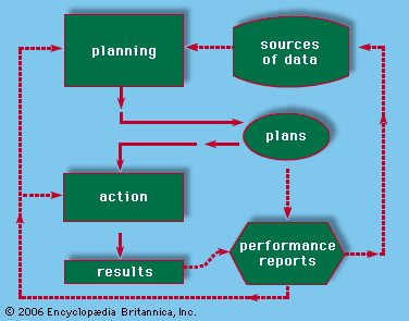
Accounting is the systematic development and analysis of an organization’s economic affairs. It is not merely number-crunching. It is the process of creating a picture of where a company stands and where it is heading. Managers use this data to control operations. Owners use it to appraise performance. Lenders and suppliers use it to decide how much credit to extend. Governments use it to determine tax liabilities. Even customers may look at the books when contracts require cost-based pricing.
The output of this process falls into two buckets. Most of it is historical. The accountant records what has already happened. They observe activities, record their effects, and summarize them in reports. The rest is predictive. These are forecasts and plans for current and future periods.
Accounting applies to any entity. It tracks the economic operations of entire countries. This article focuses on business accounting.
The Objectives and Characteristics of Financial Reporting
The main goal of financial reporting is to provide useful information to investors, creditors, and other interested parties. The ideal accounting system helps stakeholders predict the amounts, timing, and uncertainty of future cash flows. It also discloses details about economic resources and the claims to those resources.
Stakeholders now demand more than just numbers. There is growing pressure for information about social impacts. Companies increasingly report on environmental risks, employee conditions, community involvement, and consumer safety. Much of this reporting remains voluntary, particularly in the United States.
Quantitative data is now supplemented by precise verbal descriptions of business goals. In the US, publicly traded companies must include a “management’s discussion and analysis” (MD&A) in their annual reports. This document summarizes historical performance. It also includes forward-looking information.
For accountants, two characteristics define useful information.
- Relevance
- Reliability
Relevance means the information can potentially alter a decision. It helps improve predictions of future events. It confirms the outcome of previous predictions. It must be available before a decision is made.
Reliability means the information is verifiable, representationally faithful, and neutral. Neutrality is the key. Accounting information should not be selected to benefit one class of users while neglecting others.
There is a tradeoff between relevance and reliability. But information lacking either is considered insufficient for decision-making.
Accounting information must also be comparable and consistent. Comparability allows you to compare two companies in the same industry at a single point in time. Consistency allows you to compare the same company over a period of time.
Financial reporting should generally satisfy the full disclosure principle. Any information that could influence an informed decision-maker should be disclosed clearly in the financial statements.
Company Financial Statements
The primary output of financial accounting is the annual financial statement. It contains three main components.
- The balance sheet
- The income statement
- The statement of cash flows
In some jurisdictions, summary financial statements are available or required quarterly. These reports are sent to investors and others outside the management group.
Some companies post these statements online. In the United States, public corporations can be accessed through the Securities and Exchange Commission (SEC) website. The preparation of these reports falls under financial accounting.
Economists see income differently than accountants. For economists, income is simple. The change in an asset over a period of time. Does not include funds added or withdrawn by the owner. It measures how much a company can spend today while keeping its actual assets unchanged at the end of the year.
Let’s look at a basic example. If net worth increases from $1,000 to $1,200 and the company pays a $100 dividend, the economic income is $300. Get the final value ($1,200), subtract the starting value ($1,000), and add back what was taken out ($100). It is very beautiful. It is based on values.
Accountants dispute this. They found “value standards” too confusing. We rely too much on future speculation. Future value is difficult, if not impossible, to independently verify. That’s why they use a “transactional approach”.
The Transaction Approach to Income
In this system, revenues are only recognized when a genuine transaction with an external party takes place. Revenue is recognized when the work is completed, the goods delivered and the customers are invoiced. It’s not about “how much” something is worth. This is about what really happened.
This method requires two types of estimates.
- Revenue estimates: How much money do you get?
- Expense estimates: What resources were used to generate this income?
Estimating income is half easy. But it still carries judgment. The biggest risk is bad debts. You need to estimate how much of the total sales will go unpaid. Customers cannot pay. We can also return defective products. You must anticipate this loss.
Estimating costs is more complicated. These are usually based on historical costs. Net income is essentially the difference between the income received and the cost of resources consumed. The most difficult part is to determine how much of the asset’s cost was spent during this period.
Depreciation and property value
Not all assets disappear at once. Some wear out over time. This is where depreciation comes into play.
Depreciation is the cost of the part of an asset that is used to generate income over a period of time. In the balance sheet, the assets are shown at the original acquisition cost less depreciation. This allowance represents a percentage of the total economic life of the used asset.
To estimate depreciation costs, you need to anticipate two things:
* The time during which the asset provides a useful service.
* Service capacity used for each period.
Accountants rarely use complex physics to solve this problem. They use a simple formula. The two most common are:
- Straight-line depreciation: Record the same amount of expenses each year. It’s predictable and boring.
- Declining-charge depreciation: Record more expenses in the early years than in later years. Here, the assumption is that the asset’s value or efficiency will decrease over time.
These estimates are verified by independent auditors. Their job is to make sure the formula is stable and applied consistently year after year. If the company changes its approach unreasonably, these numbers lose their meaning.
Cost of goods sold and inventory
Depreciation is not the only accounting that has multiple measurement principles. Cost of Goods Sold (COGS) follows a similar logic.
Calculate cost of goods sold by starting with the total cost of goods available for sale. This is the sum:
1. The cost of beginning inventory.
2. Product purchase costs during the period.
Next, we need to divide this amount. This can be divided into the cost of goods sold and the cost of the ending inventory. Depending on how you value your ending inventory, your cost of goods sold (COGS) amounts may change. This changes the net income. The amount of tax you pay changes accordingly.
The choice of inventory valuation method (FIFO, LIFO or weighted average) is important. Each treats the transfer of goods differently. Each impacts the result.
“Revenue is measured when the external customer work is finished, the goods are delivered or the customer has been invoiced.”
This statement represents the accountant’s belief. It’s not about potential. It’s about transaction. But even this deal is based on estimates. bad debts. Asset life. Inventory flow.
The numbers in the annual reports look strong. They are precise to the cent. But they are based on speculation about the future. These assumptions must be understood. Otherwise, what you are reading is fiction disguised as fact.

Accountants use three main methods to reduce inventory costs. First in, first out (FIFO). It is last in, first out (LIFO). and average costs.
LIFO is widely used in the United States. The Internal Revenue Service (IRS) also accepts it for income tax purposes. What about most other countries? They stick to FIFO or average cost variation.
Here’s the problem. Average cost and FIFO produce very similar results. So when trying to understand how prices change between books, just look at FIFO and LIFO.
How First In, First Out (FIFO) actually works
Create a new batch every time you buy a product. Each lot has a special price tag.
First-in, first-out cost of goods sold (COGS) is not a guess. This is a calculation. You can start with your oldest inventory. Then add the old one. Continue until the sales volume is reached.
Out of stock? This will give you the price of the last batch purchased. This is the last one.
Think of a grocery store. The milk on the bottom shelf is older than the milk on the top shelf. Sell the old milk first. This is what FIFO does.
Specific examples
Let’s look at the numbers. Real number.
Let’s say your original inventory and purchase situation are as follows:
- Lot A: 100 pieces, $10 each
- Lot B: 100 pieces, $12 each
- Lot C: 100 pieces, $14 each
If you sold 150 units, FIFO means you sold:
– Lot A 100 pieces (US$1,000)
– Lot B, 50 pieces ($600)
The cost of goods sold is $1,600.
What is your final stock? This includes the remaining 50 units of Lot B and all 100 units of Lot C. These are the most recent costs.
This is important. Why? This is because in an inflationary environment, FIFO reduces cost of goods sold. Older, cheaper numbers are used. This means that reported profits will increase. But it also means raising taxes.
The opposite of the LIFO rule. Use the most recent and most expensive price figure for products sold. Profits will be smaller. lower taxes.
Your net profit will vary depending on the method you choose. This changes the amount of tax to be collected. It changes investors’ perception of the company’s efficiency.
There is no “right” answer. The options are just different.
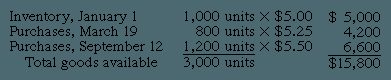

The status of your ending inventory varies depending on the accounting method you use. FIFO (first in, first out) means that the oldest leaves the building first. So the newest one stays on the shelf.
In this case, the company transferred 1,900 units. There are also 1,100 units in stock.
FIFO assumes that the first item purchased is the first item sold, so the remaining 1,100 items are valued at the most recent purchase price. That price is $5.50 per unit.
Therefore, the ending inventory value is:
1,100 units x $5.50 = $6,050
It’s very simple. The “last” purchase remains in the accounting. The “first” purchase becomes the cost of goods sold.
Why does LIFO flip the script?
Next, let’s look at LIFO (last in, first out). This method assumes the opposite. The assumption is that the newest products are sold first.
This matters. A lot.
With LIFO, your current costs against current revenue. In the LIFO method, cost of goods sold consists of recent purchases first. Then the next most recent. Keep stacking until you reach the total number of sales.
Here the total is 1,900 units.
Therefore, there is no need to look at old inventory to find LIFO cost of goods sold. You look at the latest buys. Start with the most recent purchase date and add the amount backwards until you have counted 1,900 items.
What is the main difference? FIFO leaves the newest, most expensive products in stock. LIFO immediately pushes these new costs into the expense column.
As prices rise, LIFO show higher expenses and reduces taxable income. With FIFO, expenses will show lower and reported profits are higher.
The mechanism is simple. It’s just about which units you declare as “sold” first.
In the FIFO example, we know the ending value of the inventory ($6,050). If necessary, you can calculate the cost of goods sold back.
Use LIFO to start with the sales quantity (1,900 units) and apply the most recent price to that. The calculation follows the purchase schedule in reverse order.
The result is COGS data that reflects recent market prices rather than historical costs at the beginning of the year.

Estimating ending inventory using the LIFO method
The last-in, first-out (LIFO) method reverses the calculation. The products we sell are the latest products. The items left on the shelves are the oldest. This creates a special balance sheet value.
The ending inventory cost reflects the price of the oldest available unit. It does not reflect current replacement costs. It all goes back to the beginning of this year. Or further.
Let’s consider a simple scenario. The company started with 1000 units. Price $5 each. That’s $5,000.
They buy more all year round. One purchase includes 100 pieces priced at $5.25. That adds $525 to the total.
If your company has used LIFO since day one, the ending inventory consists of the first 1,000 items. Plus the 100 units from the first purchase. The total is $5,525.
Why is this important? Because inflation raises prices. LIFO keeps older, cheaper costs in inventory. New and higher costs are transferred to cost of goods sold. This reduces taxable income. But it also means that inventory looks smaller on paper. You don’t know the true present value of what you’re leaving behind.
This method can distort comparisons. Companies that use LIFO look different than companies that use FIFO (first in, first out). The value changes depending on the time of purchase. when selling.
Why multinational companies need a common financial language
Capital does not care about borders. But there are rules behind it.
Uniform accounting standards are essential for the proper functioning of the global economy. It’s not just about the spreadsheet looking good. This aims to reduce the huge costs of doing business across borders and make international markets really efficient. Money moves faster when investors can compare like with like.
This pursuit of consistency does not happen in isolation. It is driven by the rise of multinational companies and the explosive growth of international capital markets. Consider the collapse of the Soviet Union and the creation of the European Monetary Union or NAFTA. These changes force LDCs to open their doors and speak the same economic language as other countries in order to attract foreign investment.
The numbers still don’t add up
Even today, the technical differences are obvious. You wouldn’t know it from the headlines, but the way countries value assets can change the overall picture of a company’s health.
In Great Britain, property prices are usually determined by current market prices. Stateside? This was considered too unreliable. We stick to historical costs. If you bought a building in 1950, its book value is the 1950 value, not the current value.
Then there’s Japan. Their pension calculation focuses on cash flow. Us? We are obsessed with future debt.
These are not minor quirks. They can affect the value of securities, inventories and even goodwill. Some jurisdictions give companies wide discretion in choosing their rules. Others are difficult. The differences in deferred taxes, leasing payments and research costs are enough to make it difficult for auditors.
Disclosure and enforcement: hidden barriers
The biggest hurdle isn’t just math. This is culture.
Financial reporting is a mirror that reflects a country’s legal system, language and economic history. Germany and Japan have historically required much less disclosure than the United States and Great Britain. Why? Because their economies depend on the capital of a few big banks. If the banks know what’s going on, the public doesn’t need to know.
But things have changed. Regulations are tightening as European and Japanese companies begin to raise capital from a wider pool of investors. Governments in both regions recognize that openness is essential to the functioning of modern capitalism. The reporting requirements have become stricter.
But enforcement efforts are patchy. Some countries actively regulate books. Some people let companies slide. This makes it almost impossible to compare the “quality” of cross-border income without detailed forensic accounting.
The fight for transnational standards
National standards are so entrenched that truly “international” accounting didn’t just appear. It was built by a group trying to connect these disparate systems together.
Key players are brought in to handle heavy tasks.
* International Federation of Accountants, headquartered in New York, representing 114 professional societies.
The International Accounting Standards Committee (IASC) was founded in London in 1973.
* Organization for Economic Cooperation and Development (OECD).
European Economic Community.
IASC is a pioneer. In 2001, it evolved into the International Accounting Standards Board (IASB) and assumed responsibility for the next phase of coordination.
How the IASC and IASB are changing the game
Progress is slow, but steady. By 1999, the IASC had drawn up a list of “core standards”. These are not just suggestions. These are becoming the de facto rulebook of global finance.
Early adopters were forced to follow. The London and Hong Kong stock exchanges require foreign listed companies to comply with IASC standards. This is a huge win for standardization.
The political pressure is also real. The finance ministers of the G7 countries (Canada, France, Germany, Italy, Japan, Great Britain and the United States) have approved these standards. They want uniform rules.
This pressure has real consequences for the United States. The Financial Accounting Standards Board (FASB) has eliminated the controversial “pooling of interest” for business combinations. This approach allows companies to merge without recognizing certain costs, making it difficult for investors to understand the true costs of the acquisition. Eliminating it would bring US GAAP closer to IASC standards. The American Institute of Certified Public Accountants publicly supports the IASC’s efforts to seek enforceable global rules.
The voluntary trap
But let’s be clear: this problem is not yet solved.
Despite the attention that the IASB standards received at the beginning of this century, the United States held its position. Foreign companies listed in the US must still adjust their accounting to US GAAP and not to the recommendations of the International Accounting Standards Board.
In addition, compliance with IASB standards is still voluntary.
Voluntary standards cannot be enforced. If Brazilians or Brazilian companies decide to ignore the basic standards, there are no teeth to make them comply. This creates a two-tiered system. We are a company group that follows transparent and high-quality rules. Play with others.
Until it is mandated and widely implemented, global accounting will remain fragmented. All investors can do is translate between dialects instead of reading a single language.
The change mechanisms are already ready. The standards are written. But without legal enforcement, they are just guidelines. In the financial world, guidelines are often seen as recommendations.
The International Accounting Standards Board (IASB) faces a structural blind spot. The rules themselves are often criticized for being too broad. Interpretive guidelines lag behind the actual standards. This leaves a lot of room for ambiguity. Companies and auditors can only guess at the details.
The IASB does not have the infrastructure to ensure enforcement.
This is not just a theoretical question. It is a practical hurdle. Without clear explanations, consistency suffers. Two companies in different countries can apply the same standards in completely different ways. The intent is uniformity. Reality is fragmented.
Sovereignty and resistance
The issue has a political dimension. This is not just a technical accounting issue. Jurisdictions assert their authority. Many governments are not willing to give up control. They consider the setting of accounting rules to be a matter of national sovereignty.
An international body cannot easily override local laws. This creates friction points. Some regions may adopt these standards, but with significant local modifications. Some may be against it altogether. The goal of a common global standard runs into obstacles of national pride and regulatory independence.
The infrastructure is empty
The lack of enforcement infrastructure is a key limitation. The IASB sets the rules. It does not police them. There is no global accounting police. This means that compliance depends on local regulatory authorities. These regulators vary in their willingness and ability to enforce.
This creates a patchwork system. In some places, the IASB’s rules are taken seriously. In other cases, they are ignored or distorted. As a result, “global” standards are rarely truly global standards. It is a collection of local interpretations held together by hope.
Why this matters to investors
For investors, this ambiguity is dangerous. This makes comparisons difficult. If Company A in Europe and Company B in Asia report their earnings using similar IASB rules, their numbers may not be comparable. The interpretations differ. The enforcement differs.
The lack of comprehensiveness in the guidance means that users of the financial statements must read between the lines. You can’t just rely on standards. They have to dig into the notes. They need to understand the local situation. This adds a level of due diligence that is often overlooked.
The IASB’s goal is convergence. But without implementation and clear explanations, convergence is aspirational. Not true. The gap between the rules and reality is still large.
The hidden calculations behind product pricing
You can’t put a price on something you don’t understand. Figuring out costs is the boring engine room of business planning. This is how companies estimate the costs of manufacturing a product, servicing or even maintaining a certain department. Some numbers remind us of what happened. Some predict what will “happen”. But they all follow the same rules. This means that the costs assigned to an object (work, product, process) must correspond to all the costs actually incurred for that object.
If the products are identical: Process costing
If you are making cement or grinding flour, the result will be even. You don’t need to track every bag of flour. All you need to do is know your total bill for the month and divide it by the total number of bags produced. This is the process cost. This is the simplest costing method because it assumes uniformity. You can collect costs for each production activity in a specific time period. This amount is re-averaged by dividing total costs by total production.
This only works if the individual processes produce fairly consistent products. This is continuous production. It is based on quantity. It’s very simple. But what if you do custom work? This method failed.
Customized work tracking: Work order costing
If your department processes multiple products instead of a single Stream, you can switch to job-order costing. Here, factory costs are divided into two categories: prime costs and overhead.
Prime costs are direct costs. Can be traced to a specific lot or job lot. Direct labor. direct material. These are entered directly into the cost table of the work order.
Overhead is the messy stuff. It cannot be tied to one job. The salary of the department supervisor? Overhead. The electricity for the whole floor? Overhead. Use overhead to allocate these costs. It is the ratio of overhead rates to total production over a period of time.
Allocating the invisible costs
You can calculate separate overhead rates for each manufacturing department. If your departments have varied operations, you can divide them into more homogeneous cost centers, each of which has its own prices. Sometimes it goes even deeper. If the operating costs of individual machines differ significantly in terms of power consumption, maintenance and depreciation, it makes sense to apply separate rates.
The production of these centers is not uniform, so you cannot just count the units. Output can be measured in machine hours or direct labor hours. Once you’ve determined this price, you can add overhead to each job.
Example: If overhead is $3 per machine hour and job number 7128 uses 600 machine hours, allocate $1,800 of overhead to this job only.
But wait. There is also a support department. Maintenance. Quality control. clean. Power production. These are not used to create products. They support those who do. Estimate and allocate costs to production departments based on the proportion of services received by each department. These allocated costs are taken into account in the department’s overhead rates.
In addition to quantity: activity-based costing
What if the costs do not increase as the quantity of the product increases? Enter Activity Based Costing. This approach recognizes that many costs are caused by factors other than production volume. The first step is to identify the activities that generate costs. The cost of each activity is then estimated and expressed as an average value per activity unit.
Managers can use these averages to reduce waste. If you want the price of a specific product, you can estimate the number of activity units in use for that product and multiply it by the average cost.
Consider a product assembled from six parts. It costs $100 per year per component to maintain it in the product line. That’s $600 a year regardless of the amount. Even if you produce nothing, you still have to pay $600.
Add batch costs now. If your costs driven by production batches an average of $100 per batch, using a batch of 1,000 units costs $0.10 per unit.
Add machine time. If hour-driven costs average $12 per machine hour and a batch requires 15 hours, that’s $180 per batch. Divide by 1,000 units and you get $0.18 per unit.
If production is 10,000 units, the product’s maintenance cost is $0.06 per unit. The batch cost is $0.10. The machine cost $0.18. All? $0.34 per unit. Add the materials. It also includes other hidden activities that you haven’t followed yet.
Does your current pricing model take into account the cost of maintaining your product line, or are you just making assumptions based on labor and materials? The difference between profit and loss is often in the details that others don’t notice.
The reality of the Pre-Production Estimates
Knowing the true cost of a product before it is manufactured rarely requires simple addition. This is mostly an educated guess. Whether you use activity-based costing, process costing, or job order costing, you may be using estimates instead of actual receipts.
Process costing allocates costs as production moves. Job-order costing records the amount spent on a specific job. However, the problem here is that the overheads used in both methods are usually predetermined. These reflect a average planned overhead.
Why? This is because the actual overhead costs depend on the overall operational efficiency and peak volume. These are external variations. They are not limited to one job. If these variations change the overhead allocated to a particular job, the cost information becomes irrelevant. You end up with noise instead of signal.
Many companies go further. They don’t just estimate. They create routine estimates for all types of materials, every operation and all products. These are standard costs. Your number is easily accessible when you need it. These also serve as a benchmark for performance reporting later on.
Services Have Costs Too
This does not only apply to factories. Service providers use similar methods to find out and estimate costs.
Think of an advertising agency. Or a consulting firm. They maintain job cost records. This is done to ensure accurate invoicing of customers. This is also done to assess the profitability of individual accounts. The mechanism is the same. Track your input. You assign rates. You see if the margin holds.
Full Costing Versus Variable Costing
The above method is called full costing or absorption costing. Overhead includes provisions for “all” manufacturing costs.
These same methods can be adapted to variable costing. In this model, only variable manufacturing costs are included in product costs.
The behavioral differences are as follows:
– Variable costs rise or fall according to production.
– Total fixed costs remain constant (in the normal range) at different volume levels.
In variable costing, the unit cost is simply the average variable cost of producing the product. It is often more useful than average total cost for short-term business decisions.
Consider choice to manufacture goods in large lots. Management must estimate the cost of larger finished goods in inventory. Increasing inventory causes more variable costs. Fixed manufacturing costs are generally unaffected.
When a decision causes a change in a firm’s fixed costs, the change is rarely proportional to volume. Average fixed costs are not a sufficient basis for evaluating the cost effects of such decisions. Variable costing removes the temptation to use average fixed costs instead of variable costs.
The GAAP Trap
Even if you use variable costs for internal decision making, you still need to track fixed overhead. provide supplemental rates for fixed overheads. This is necessary to measure the costs allocated to year-end inventory.
Why is this additional step necessary? Generally accepted accounting principles (GAAP) in the United States and most other countries require that, in external financial reporting, inventory is valued at the full cost of the product.
You cannot avoid the attention of tax authorities and shareholders. But what if manager staring at a pricing dilemma? Variable costs bring clarity. Remove the noise. Leave only the parts that move according to the volume.
The alternative is clear. Get accurate external reports and complete cost accounting. Variable costs help you make better decisions in your business. You have to live with both.